Bandwidth Plot with purrr + ggplot2
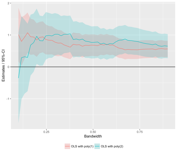
Posted: February 14, 2017 Filed under: Post | Tags: R Leave a commentRDD estimates are sensitive to bandwidth choices which is why one typically plots them for different bandwidths. Here is some code to quickly obtain RDD estimates for different bandwidths and plot the results. The code relies on the amazing purrr package.
library(purrr)
library(ggplot2)
library(dplyr)
library(broom)
library(stringr)

# Define a helper function that gives back local linear
# regression estimates when handed a bandwidth and a specification
get_lm_bw_est <- function(df,bw,formula) {
		return(  df %>% filter( abs(runningvar) <= bw ) %>%
		do(tidy(lm(formula, data=.))) %>%
		filter(term=="treat") %>%
		mutate(bw=bw, spec=format(formula) )  )
		}

set.seed(42)

# Sim Data
x <- runif(1000,-1,1)
y <- 5+ 3*x + 0.5*(x>=0) + rnorm(1000)

fakedata <- data.frame(y=y,runningvar=x, treat=as.numeric(x>=0) )

# Set up grid of specification choices and bandwidths
spec1 <- y ~ treat * runningvar
spec2 <- y ~ treat * (runningvar + I(runningvar^2))
spec <- c(spec1,spec2)

simframe <- expand.grid(bw=seq(.1,.9,length=50), spec=spec)

# Estimate, i.e. map simframe values to helper function
m <- with(simframe, map2_df(bw, spec, ~ get_lm_bw_est(fakedata, .x, .y) ))

# Calculate 95% CI and plot results
m <- m %>% mutate(lo=qnorm(0.975)*std.error + estimate,
				  hi=qnorm(0.025)*std.error + estimate)

m <- m %>% mutate(spec=str_count(spec, "running"),
				  spec=paste("OLS with poly(", spec, ")", sep=""))

ggplot(m, aes(bw,estimate,group=spec)) +
	geom_ribbon(aes(ymin=lo,ymax=hi, fill=spec), alpha=0.25) +
	geom_line(aes(colour=spec)) + geom_hline(aes(yintercept=0)) +
	theme(legend.position='bottom', legend.title=element_blank()) +
	ylab("Estimates / 95%-CI") + xlab("Bandwidth")
Zero-Numerator Problem: Calculating the Expected Number of Mistakes in Data Entry Jobs
Posted: January 1, 2017 Filed under: Post | Tags: Bayesian, data entry, R, research practice Leave a commentI have a project for which I need to digitize a series of tables from scanned pdf pages. Due to the scan quality, some pages are handled manually by research assistances. After receiving a new badge, I typically like to estimate how many data-entry errors I have to expect. Therefore I draw a random evaluation sample and carefully check if the entered numbers matches the originals in the pdf. Depending on the sample size and the quality of the badge, I often arrive at a count of zero errors for the evaluation sample.
What does a zero count for the evaluation sample say about the distribution of errors in the entire badge? If the sample is randomly drawn, the number of errors, F, has a Bernoulli density with parameter S and p. The parameter S denotes the number of checked cells (the sample size) and p measures the true proportion of incorrect values across all cells. While S is known, p is not and constitutes the estimand.
A typical estimator for p is the sample mean, but in the event of F=0, the estimate for p is 0 for any sample size. That is, the sample mean estimator always suggests that the expected number of errors is zero — independent of the size of the evaluation sample. The same holds for an interval estimator of the 95% confidence interval. In the event of zero errors, the estimate for the sample variance is also ‘0’ and consequently the 95% confidence interval is zero regardless of the sample size.
A version of this problem is well-known in the bio-statistical literature. The task here is to compare two procedures (or treatments): One for which the risk of people being harmed (killed) is well-known and another for which only sample information with not a single harmed individual is available. The standard approach seems to be to calculate the upper bound of the 95% confidence interval using 3/S as an estimator (also known as The Rule of Three).
As pointed out in several contributions — for a summary see Winkler et al. (2002)
— a more principled way to form an estimate requires Bayesian Statistics and starts with the assignment of an informed prior density over p. This prior is then updated using the newly gathered data point ‘0 errors in an evaluation sample of size S’. To the extend that the prior is expressed as a Beta distribution, the calculations are algebraically easy.
However, the tricky part is typically to come up with a reasonable prior density for p. In practice, I make use of some very old numbers reported in a paper by Baddeley and Longman (1978). Back in the days when post codes had to be manually typed, they conducted an experiment with groups of postmen to evaluate what type of training procedures reduce the number of wrongly typed “alpha-numeric code material”.
In the table below I reproduce the Baddeley-Longman numbers and also the variance I calculated from the range estimates. Averaging across the four groups suggests that the rate of errors is about 1.4% with a variance 0.7. A more conservative set of estimates might be stipulated from using the values reported from group 4 alone (2.1 for the mean value and 1.1 for the variance).
| Group 1 | Group 2 | Group 3 | Group 4 | |
|---|---|---|---|---|
| % Incorrect | 1.09 | 1.14 | 1.41 | 2.06 |
| Range | 0.22 – 2.18 | 0.06 – 2.42 | 0.40 – 3.45 | 0.38 – 4.65 |
| N | 18 | 18 | 18 | 18 |
| Variance | 0.49 | 0.59 | 0.76 | 1.07 |
Using these values, it is easy to calculate the implied Beta prior and the posterior distribution and its characteristics when combined with the information from the evaluation sample. In Bayesian Statistics the calculations are known as Beta-Binomial update.
In order to simplify these calculations, I have written a short R function that makes the calculations when given information about the evaluation sample. The user can choose between the two pre-programmed priors mentioned above or supply its own. The function is part of my datatools package and can be installed from my github, via devtools::install_github('sumtxt/datatools').
As an example, suppose we have an evaluation sample of S=20 with F=0 (no errors). Using the function, we find that the expected proportion of errors in the population is about 1.3% and the upper bound of the 95% credible interval equals 2,5%.
datatools::est_typing_err(20, F=0, prior='postmen', quantity='mean')
[1] 0.01306888

datatools::est_typing_err(20, F=0, prior='postmen', quantity='95q')
[1] 0.02538156
Notice: These estimates differ from the estimates implied by the sample-mean estimator (0%) and the rule-of-three estimator (3/20=15%).
IR dyad-year dataset with 10 lines of dplyr + tidyr code
Posted: July 29, 2015 Filed under: Post | Tags: dplyr, International Relations, IR, R, tidyr 2 CommentsDirected (country)-dyad-year datasets are quite common in International Relations (IR) research and from time to time one requires an empty one. Creating this used to be a hassle with +50 lines of code (see example in PERL or R). Luckily, with tidyr + dplyr + pipping building such a dataset requires at most 10 lines of code:
system <- read.csv("./raw data/states2011.csv")
system <- system %>%  select(ccode, styear, endyear)
system <- system %>%  expand(statea=ccode, stateb=ccode, year=seq(1816,2011)) %>%
				  filter(statea!=stateb) %>%
				  left_join(., system, by=c("statea"="ccode")) %>%
				  filter(year >= styear & year <= endyear) %>%
				  select(-styear,-endyear) %>%
				  left_join(., system, by=c("stateb"="ccode")) %>%
				  filter(year >= styear & year <= endyear) %>%
				  select(-styear,-endyear)
First, the code block creates all possible country-country-year pairings (line 3) and then filters out the dyad-years which are inadmissible either because a) the dyad involves the same country (line 4) or b) at least one of the dyad-members does not exist in a particular year (lines 5-10).
Data Source: Correlates of War System Membership 2011
Tricks for working with JAGS
Posted: May 8, 2015 Filed under: Post | Tags: BUGS, JAGS, R Leave a comment- The Gamma distribution is frequently used as a prior for the precision in a model because of its conjugacy with the Normal. Given JAGS parameterization of the Gamma distribution with a rate and shape parameter, it’s not easy to select sensible hyper-parameters. It’s easier to think of hyper-parameters that correspond to the mean and the variance of a prior for the precision. To use mean and variance hyper-parameters (mu and sigma) with JAGS’s
dgamma, use:dgamma( ((mu^2)/sigma), (mu/sigma)). - The
glmmodule provides a series of more efficient samplers that JAGS automatically selects whenever possible (e.g. Albert/Chib (1993)). This usually leads to much better mixing. I tend to load the module right away with the actualrjagspackage, e.i.library(rjags); load.module("glm"). - To check which samplers are selected by JAGS, use the
list.samplers()function on the JAGS model object. This is useful, because sometimes a slight change in the coding helps JAGS to select better samplers. For example, when using a logit model in JAGS and you want the Holmes-Held sampler from the glm module to work, do not usedmnorm()butdnorm()for the prior of the coefficient, e.i. do not use blocking. - Avoid deterministic nodes as much as possible to increase speed. In particular, do all pre- and post processing in R including drawing from the predictive distribution and compute deterministic functions inside probabilistic statements, e.g.
y ~ dnorm( (x*beta), 1)instead ofmu . - For comprehensible / readable code, let the running index be the small letter corresponding to the capital letter of the upper limit, e.i.
for(n in 1:N)instead offor(i in 1:N). This becomes especially useful when one has many nested hierarchies.
Gibbs Samplers in R and Notes
Posted: May 4, 2015 Filed under: Post | Tags: MCMC, R Leave a commentI uploaded several R files and notes for Gibbs samplers to my Website’s resource page. They include: Factor Analysis, Finite Mixture of Linear Regression Models and Probit Regression. I have written all this a while ago when I was reading about these models. Most of the samplers are fairly standard and well-implemented efficiently in R packages calling c++ in the background. These packages are also referenced in the R files. Nevertheless, the R code might be useful for pedagogical purposes or as building block for more complex schemes.
Generate a panel version of the UCDP/PRIO Armed Conflict dataset
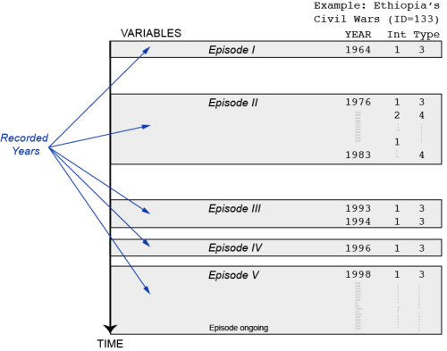
Posted: October 30, 2013 Filed under: Post | Tags: data, R, UCDP 1 CommentI spent the morning writing a short R script that transforms the UCDP/PRIO Armed Conflict dataset into a panel dataset in which each conflict is observed from the year it started to the year it ended (or the last year in the dataset). The unit of observation in the original dataset is an active conflict observed in a year t. More precisely, it is an ongoing conflict episode (for a particular conflict) in a year t. Inactive years between conflict episodes are not recorded (see figure with an example from Ethiopia and two variables from the dataset). The purpose of the code below (especially the second part) is to fill-in the observations between conflict episodes. In addition to the panel structure, I wanted to have a more natural variable structure / variable names (this is what the first part is doing).
The code below might not be optimal for all applications, but it is probably still useful for others that need to get a panel version of the UCDP/PRIO. If you spot mistakes or have ideas for improvements, please share them in the comments. For an introduction to the dataset, definition of variables etc, please read the original codebook.
Read the rest of this entry »
Running Parallel MCMC without specific R packages
Posted: May 19, 2013 Filed under: Post | Tags: MCMC, R 1 CommentRunning multiple, distinct Markov chains that have a posterior density as their equilibrium density is useful to use convergence diagnostics such as the Gelman / Rubin diagnostic (Gelman & Rubin, 1992). In order to save time, one likes to run each Markov chain in parallel. There are a number of packages in R (parallel, snow,…) to run code in parallel. However, I find it more useful to write a script for a single chain and then dispatch it multiple times from the terminal. Here is an example with the MCMCpack:
Save the following as “sim.R”:
substream <- as.numeric(commandArgs(trailingOnly = TRUE))

library(MCMCpack)
data(birthwt)

filename <- paste("posterior_", substream, ".Rdata" , sep="", collapse="")
out <- MCMCprobit(low~as.factor(race)+smoke, data=birthwt,
 b0 = 0, B0 = 10, seed=list(NA, substream))
save(out,file=filename)
The first line grabs the seed argument from the terminal and pass it to MCMCprobit function which generates a single chain. The script can be executed from the terminal with four different substream seeds as follows:
Rscript --arch=x86_64 sim.R 1 & Rscript --arch=x86_64 sim.R 2 & Rscript --arch=x86_64 sim.R 3 & Rscript --arch=x86_64 sim.R 4
If you don’t have a 64-Bit machine, use “x86_32”. Provided that you have four cores, one core will be used for each of these jobs. Next, you can fuse the output together in an mcmc.list object and run the Gelman/Rubin diagnostic.
library(coda)
load("posterior_1.Rdata")
out1 <- out
load("posterior_2.Rdata")
out2 <- out
load("posterior_3.Rdata")
out3 <- out
load("posterior_4.Rdata")
out4 <- out

posteriors <- as.mcmc.list(list( as.mcmc(out1), as.mcmc(out2),
 as.mcmc(out3), as.mcmc(out4)))
gelman.diag(posteriors)
The great benefit of this approach is that the R code is less crammed with parallelization functions and the process can be monitored since the output is dumped right into the terminal window.
References
Gelman, Andrew & Donald B. Rubin. 1992. “Inference from Iterative Simulation Using Multiple Sequences.” Statistical Science 7(4):457–472.
Standard error / quantiles for percentage change in hazard rate
Posted: January 24, 2013 Filed under: Post | Tags: function, R, simulation, survival model Leave a commentBox-Steffensmeier / Jones (2004, 60) suggest in their book “Event History Modeling” to calculate the “percentage change in hazard rate” to simplify the interpretation of estimates from Cox models. The quantity is defined as:

I wrote a little R function for calculating this quantity. Since the coefficients (b) are unknown quantities and can only be estimated, the function takes into account their uncertainty and simulates a distribution of the “percentage change in hazard rate”. The output is the mean and the quantiles of the simulated distribution. Licht (2011) suggested something similar in the context of non-proportional hazard modeling.
| # FN calcualtes Box-Steffensmeier %h(t), (Box-Steffensmeier / Jones, 2004, 60) | |
| # | |
| # %h(t) = ( exp(b*X_1) - exp(b*X_2) ) /exp(b*X_2) | |
| # | |
| # Input: | |
| # - x: a vector of two values for the quantity of interest that changes from the first value to the second value | |
| # - xname: the variable name of the covariate that is the quantity of interest | |
| # - Xfix: a dataframe of all other covariate values that are kept constant | |
| # - model: the coxph model | |
| # Output: | |
| # - mean and quantiles of %h(t) | |
| # Caution: FN doesn't work with frailties or splines | |
| hazChange <- function(x,model,Xfix,xname, n=10000){ | |
| require(MASS) | |
| newdata <- cbind(Xfix,t(x)) # combine data | |
| colnames(newdata) <- c(colnames(newdata)[1:(dim(newdata)[2]-1)],xname) # assign names | |
| simdata <- model.matrix(model,newdata) # sort newdata columnes such that simcoef and simdata are matching | |
| simcoef <- mvrnorm(n=n, coef(model), model$var) # draw coefficients | |
| p <- ( ( exp(simcoef %*% simdata[1,] ) - exp(simcoef %*% simdata[2,] ) ) / exp(simcoef %*% simdata[2,] ) ) * 100 | |
| r_updow <- quantile(p, probs=c(0.025,0.975)) # calculate quantiles | |
| r_mean <- mean(p) | |
| return(c(r_mean,as.vector(r_updow))) | |
| } | |
| # EXAMPLE | |
| # colon data | |
| library(survival) | |
| library(plyr) | |
| library(Zelig) | |
| fit.model <- coxph(Surv(time, status) ~ extent+ node4*age + sex+ cluster(id), data=colon, robust=TRUE) | |
| Xfix <- data.frame( extent=c(3,3), sex=c(0,0), node4=c(1,1), id=c(1,1) ) | |
| X <- data.frame( 53, seq(54,69,1) ) | |
| out <- adply(X,1,"hazChange",model=fit.model,Xfix=Xfix,xname="age") | |
| colnames(out) <- c("min","max","hmean","hup","hdow") | |
| out$diff <- out$max-out$min | |
| plot(out$diff, out$hmean,ylim=c(-14,14), xlab="Difference in 'age'", ylab="%h(t)", pch=20) | |
| segments(out$diff, out$hdow, out$diff, out$hup,col="red") | |
| abline(h=0) | |
| # EXAMPLE | |
| # coalition data | |
| m1 <- coxph(Surv(duration, ciep12) ~ crisis + fract, coalition) | |
| Xfix = data.frame(fract = rep(mean(coalition$frac), 2) ) | |
| X <- data.frame( 0, seq(0,30,1) ) | |
| out <- adply(X,1,"hazChange",model=m1,Xfix=Xfix,xname="crisis") | |
| colnames(out) <- c("min","max","hmean","hup","hdow") | |
| out$diff <- out$max-out$min | |
| plot(out$diff, out$hmean, xlab="Difference in 'crisis'", ylab="%h(t)", pch=20) | |
| segments(out$diff, out$hdow, out$diff, out$hup,col="red") | |
| abline(h=0) | |
The working of the code is pretty simple. 1) Estimate the model, 2) Get the Hessian and coefficient vector, 3) Use them to generate draws from a multivariate normal distribution, 4) Calculate the hazard change quantity for each draw and 5) Estimate the mean and quantiles for this simulated distribution. See King et al (2000) for something similar in the context of other models.
References
Box-Steffensmeier, J. M., & Jones, B. S. (2004). Event History Modeling: A Guide for Social Scientists. Cambridge: Cambridge University Press.
Licht, Amanda A. (2011). Change Comes with Time: Substantive Interpretation of Nonproportional Hazards in Event History Analysis. Political Analysis, 19(1), 227-243.
King, G., Tomz, M., & Wittenberg, J. (2000). Making the Most of Statistical Analyses: Improving Interpretation and Presentation. American Journal of Political Science, 44(2), 347-361.
Get a slice of a mcmclist faster
Posted: July 20, 2012 Filed under: Post | Tags: BUGS, coda, JAGS, MCMC, mcmclist, MCMCpack, R Leave a commentSay you sampled a large amount of parameters from a posterior and stored the parameters in a mcmclist object. In order to analyze your results, you want to slice the mcmclist and only select a subset of the parameters. One way to do this is:
mcmcsample[,i,]
where mcmcsample is your mcmclist with the posterior sample and i the parameter you are interested in. Turns out, this function is very slow. A faster way is to use this little function:
getMCMCSample <- function(mcmclist,i){
  chainext <- function(x,i) return(x[,i])
  return(as.mcmc.list(lapply(mcmclist, chainext, i = i)))
  }
Example:
# Run a toy model
library(MCMCpack)
counts <- c(18,17,15,20,10,20,25,13,12)
outcome <- gl(3,1,9)
treatment <- gl(3,3)
posterior1 <- MCMCpoisson(counts ~ outcome + treatment)
posterior2 <- MCMCpoisson(counts ~ outcome + treatment)
posterior3 <- MCMCpoisson(counts ~ outcome + treatment)
mcmclist <- mcmc.list(posterior1,posterior2,posterior3)

system.time(mcmclist[,2:3,])
system.time(getMCMCSample(mcmclist, 2:3))
The build-in way takes 0.003 sec on my machine, while getMCMCSample gets it done in 0.001. For this little example, the difference is negligible. But as it turns out, for large posterior samples, it really makes a difference.
How to setup R and JAGS on Amazon EC2
Posted: July 8, 2011 Filed under: Post | Tags: AWS, BUGS, R, script Leave a commentYesterday I setup a Amazon EC2 machine and installed R, JAGS and rjags. Unfortunately I was unable to compile the latest version of JAGS. The configuration step failed with an error that says that a specific LAPACK library is missing. I tried to install the missing library manually but for some reason JAGS doesn’t recognize the new version. After an hour, I decided to go with the older JAGS version. Here is how I installed all three packages.
[If you never worked on an EC2 machine: Here are two [1,2] helpful tutorials how start an EC2 instance and install the command line tool on your computer to access it via ssh.]
Login via ssh. In a first step we install an older version of R. It is necessary to use the older version in order to get JAGS 1.0.4 running later. After downloading the R source file, we unzip it, cd into the folder and start installing a couple of additional libraries and compilers that we need to compile R (and later JAGS). We then configure the R installer without any x-window support and install everything. The last line makes sure that you can start R with simply typing ‘R’.
cd ~
wget http://cran.r-project.org/src/base/R-2/R-2.10.0.tar.gz
tar xf R-2.10.0.tar.gz
cd ~/R-2.10.0
sudo yum install gcc
sudo yum install gcc-c++
sudo yum install gcc-gfortran
sudo yum install readline-devel
sudo yum install make
./configure --with-x=no
make
PATH=$PATH:~/download/R-2.10.0/bin/
Next, try to start R and install the coda package.
R
install.packages('coda')
q()
Now, we proceed with installing JAGS. First, get some libraries and the JAGS source code. Unzip, cd into the folder and run configure with specifying the shared library folder. The specification of the shared library path is crucial, otherwise rjags fails to load in R.
sudo yum install blas-devel lapack-devel
cd ~/download/
wget http://sourceforge.net/projects/mcmc-jags/files/JAGS/1.0/JAGS-1.0.4.tar.gz/download
tar xf JAGS-1.0.4.tar.gz
cd ~/download/JAGS-1.0.4
./configure --libdir=/usr/local/lib64
make
sudo make install
In a last step, download the appropriate rjags version and install it it.
cd ~/download/
wget http://cran.r-project.org/src/contrib/Archive/rjags/rjags_1.0.3-13.tar.gz
R --with-jags-modules=/usr/local/lib/JAGS/modules/ CMD INSTALL rjags_1.0.3-13.tar.gz
Sources of inspiration. Here, here, here and here.
